
Stage Adaptive Item Selection Method in Multidimensional Item Response Theory
June 30, 2022
This is a matter arising from one of my papers. I want to show the potential for appling the new methods proposed in the paper into the multidimensional scenario.
I would like to skip the description of unidimensional item selection methods and response time model to make it short. Instead, the next section would begin with the introduction of the compensatory multidimensional three-parameter logistic model, following with the existing method, the new methods, and simulation study.
In the multidimensional case, the examinee's responses are determined by more than one underlying trait, which can be captured by the multidimensional IRT (MIRT) model via a $m$-dimensional latent ability vector $\boldsymbol{\theta} = (\theta_1, ..., \theta_m)'$ with $m\geq2$. One of the mainstream MIRT models is the compensatory multidimensional three-parameter logistic model (Reckase, 2009):
$$P_j (\boldsymbol{\theta})=Pr(X_j=1|\boldsymbol{\theta})=c_j + \frac{1-c_j}{1 + exp(-(\boldsymbol{\alpha}_j^T\boldsymbol{\theta}+d_j))},$$
where $\boldsymbol{\alpha}=(\alpha_1, ..., \alpha_m)'$ and $d_j$ are the discrimination parameter vector and intercept parameter for item $j$, respectivcely. Note that the scalar $d_j$ represents the easiness of item $j$. Here, the $m\times m$ Fisher information matrix for item $j$ is expressed by
$$FI_j (\boldsymbol{\theta})=\boldsymbol{\alpha}_j \boldsymbol{\alpha}_j^T \frac{[1-P_j (\boldsymbol{\theta})][P_j (\boldsymbol{\theta})-c_j]^2}{P_j (\boldsymbol{\theta})[1-c_j]^2}.$$
The reference composite (RC) method, maximizing the determinant of the Fisher information matrix at the cut score on the RC, was proposed by van Groen, Eggen, and Veldkamp (2016) for the item selection in multidimensional CCT. As more than one hypothetical construct is measured in MIRT, the abilities of an examinee are located in a multidimensional space rather than on a line. When items are allowed to load on more than one dimension, moreover, such loading structure is called within-item multidimensionality (Adams, Wilson, & Wang, 1997). This structure commonly occurs in practice, meaning that a combination of skills accounts for the response to all items. For instance, mathematics problems usually measure arithmetic computation, algebraic symbol manipulation, and reading comprehension skills (Reckase, 2009).
Facing such multidimensionality, the main goal of RC is to summarize the abilities' characteristics by projecting the $\boldsymbol{\theta}$ from the multidimensional space onto the unidimensional scale in the orientation that is best measured at the test level. The orientation of RC is related to the characteristics of the $\boldsymbol{\alpha}_j^T \boldsymbol{\alpha}_j$ matrix, and is defined by the eigenvector corresponding to the largest eigenvalue (Wang, 1985, 1986). And the $l$th elements (i.e., $l = 1, ..., m$) of the eigenvector represents the direction cosine for the angle between the RC and the $l$th $\theta$-coordinate ($\alpha_{\xi l}$). All the angles are less than or equal to 90 degrees as the sum of the squared elements in the eigenvector equals to 1. For an examinee located at the $\boldsymbol{\theta}$-space, the distance from the origin to the $\boldsymbol{\theta}$ point is $L_p = ||\boldsymbol{\theta}||$, where $||\bullet||$ is the Euclidean norm function. Hence, the angle between the ability vector and the $l$th dimension axe is given by
$$\alpha_{pl} = \arccos \frac{\theta_l}{L_p}.$$
Then, the angle between the ability vector and the RC can be obtained by $\alpha_{p \xi} = \alpha_{pl} - \alpha_{\xi l}$. Once the $L_p$ and $\alpha_{p \xi}$ have been decided upon, the projected proficiency $\xi$ on the RC can be specified as
$$\xi = L_p cos \alpha_{p \xi}.$$
The $\xi$ parameter reflects the differences between examinees along the composite of abilities. The graphic presentation of an examinee's $\xi$ for a two-dimentional scenario is provided below.
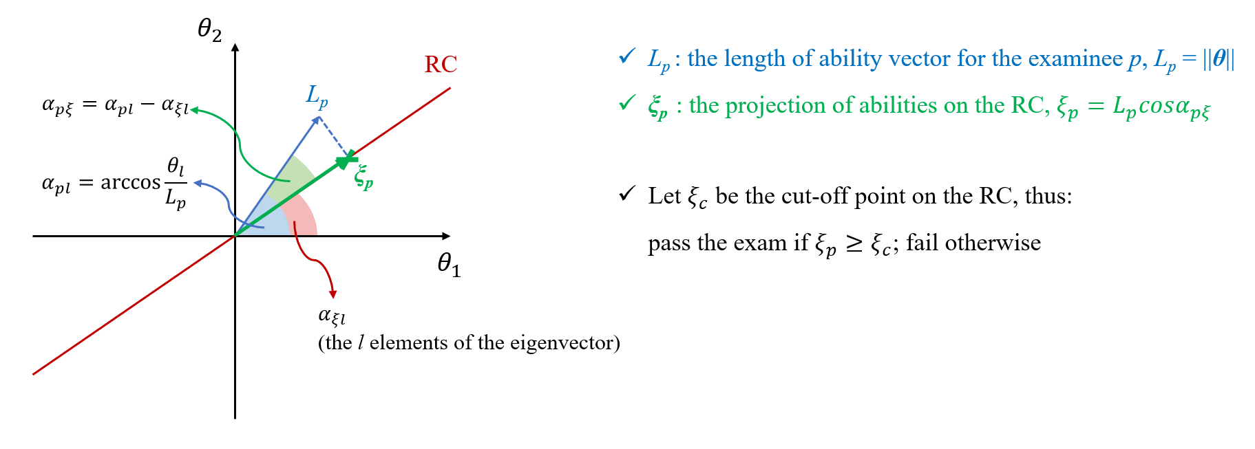
The classification decision can be made by comparing the $\xi$ with the cut score on the RC (i.e., $\xi_c$). For instance, the examinee passes the test if $\xi \geq \xi_c$ and fails otherwise.
To calculate the Fisher information matrix, the $\xi_c$ needs to be transformed into the multidimensional space using $\boldsymbol{\theta}_c = \xi_c cos \boldsymbol{\alpha}_\xi$, where $\boldsymbol{\alpha}_\xi$ is the collection of all angles between the RC and $\theta$-coordinates (i.e., $\boldsymbol{\alpha}_\xi = (\alpha_{\xi 1}, \alpha_{\xi 2}, ..., \alpha_{\xi m})^T$). Similar to the D-optimal method (Segall, 1996), the RC method selects the item $k$ with the maximum determinant of Fisher information at $\boldsymbol{\theta}_c$:
$$i_k = \arg\max\limits_{j\in R_{k-1}} {det(\sum_{i=1}^{k-1} FI_i (\boldsymbol{\theta}_c) + FI_j (\boldsymbol{\theta}_c))},$$
where $\sum_{i=1}^{k-1} FI_i (\boldsymbol{\theta}_c)$ describes the information accumulated after the first $k - 1$ items, and $FI_j (\boldsymbol{\theta}_c)$ denotes the information of item $j$ from $R_{k-1}$. Thus, the implementation of the RC method will yield the largest decrement of the confidence ellipsoid volume at the cut-off point.
In unidimensional case, the SAI method selects the item maximizing the SAI index as item $k$:
$$SAI=exp{-|r[FI_j (\theta_c )]+w\times s-1|};$$ $$i_k=\arg\max\limits_{j\in R_{k-1}}SAI,$$
In MIRT case, the equations above become:
$$SAI=exp{-|r[det(\boldsymbol{\theta}_c)_{RC}]+w\times s_{RC}-1|},$$
where $r[det(\boldsymbol{\theta}_c)_{RC}]$ and $s_{RC} = |\frac{\hat{\xi} - \xi_c}{range\ of\ RC}|$ stand for the percentile rank of the determinant of the Fisher information and the decision-making requirement based on the RC method, respectively. The length of RC can be simplified as $8/max(cos \boldsymbol{\alpha}_{\xi})$ given a well-defined region(i.e., [-4, 4]) for each $\theta$-coordinate.
To investigate the performance of the new methods in the multidimensional scenario, simulations were run for the RC, SAI, timed-RC, and timed-SAI methods (the detailed description of the timed versions can be found here). All items were designed to load on three dimensions, and three truncated lognormal distributions were used to generate the discrimination parameters for each dimension, that is, $log(\alpha_{jl}) \sim N(0,1)$ with $\alpha_{jl} \in (0.2,2.5)$ (Chen, Wang, Xin, & Chang, 2017). Therefore, the angles between the RC and $\theta$-coordinates $\boldsymbol{\alpha}_{\xi} = (\alpha_{\xi 1},\alpha_{\xi 2},\alpha_{\xi 3}) = (53.868, 57.037, 53.352)$. Following the procedures of Man, Harring, Jiao, and Zhan (2019), the ability vectors $\boldsymbol{\theta}$s for 1,000 examinees were drawn from a multivariate standard normal distribution with covariances fixed to 0.3, and the relationship between ability and speed was identical as the setting in my pervious paper. Also, the easiness $d_j$ and time density $\beta_j$ were generated from a bivariate normal distribution with mean vector of $\boldsymbol{\mu}_\Gamma = (\mu_d,\mu_\beta) = (0,4)$ and covariance matrix of $\Sigma_\Gamma = \left[\begin{matrix} 1 & 0 \\ 0 & 0.25 \end{matrix}\right]$.
Similar to van Groen et al. (2016), the cut score was set to 0 on the RC, and test length was 30. Based on the results shown in previous studies, the weighting parameter was set to 1, and the centering parameter was set to $v = {1, e^{\mu_\beta - \mu_\tau}/2}$ which resulted in $lnv = {0.0, 3.3}$. As suggested by Nydick (2013), the constrained MLE was used for ability estimation, confining the space of abilities to $\boldsymbol{\theta} \in [-4,4] \times [-4,4] \times [-4,4]$. And the first four items were randomly selected. The average for the mean and standard deviation of test-taking time, PCC, and the $\chi^2$ statistic were calculated over 100 replications.
Table 1 presented the evaluation results for different item selection methods under varying $v$ values. In general, the SAI method did equalize the item exposure rates better than the RC method with shorter and more stable test-taking time and acceptable PCC. And the two timed-methods achieved a significant reduction of the mean and SD for test-taking time, but with slightly lower PCCs. Again, the center parameter v showed a larger impact on $\chi^2$ than on the test time and PCC, indicating that the compensation of $v$ could remedy the gap between time density and speed. Unlike the unidimensional case, the timed-SAI method possessed slightly higher PCC but little poorer time control ability than the modified timed version.
Table 1. Evaluation results for four item selection methods.
| PCC | $\chi^2$ statistic | mean of test time | SD of test time | ||
| RC | 0.909 | 396.924 | 3754.538 | 4581.262 | |
| SAI | 0.901 | 23.979 | 3464.855 | 4227.865 | |
| $v=1$ | timed-RC | 0.892 | 390.863 | 1552.895 | 1907.627 |
| timed-SAI | 0.897 | 332.325 | 1621.848 | 1992.096 | |
| $v= \frac {e^{\mu_\beta - \mu_\tau}}{2}$ | timed-RC | 0.887 | 100.897 | 1719.759 | 1806.634 |
| timed-SAI | 0.892 | 93.167 | 1760.304 | 1892.445 |
Note. RC = reference composite method, SAI = stage adaptive method, PCC = percentage of correct classifications, SD = standard deviation.
The simulation results show that the newly proposed item selection methods can counterbalance the item usage and shrink the deviation and cost of test-taking time at the expense of negligible classification accuracy in multidimensional scenario.
It should be noticed that this study is limited to the within-item multidimensionality structure as the non-diagonal elements of the discriminating parameter matrix $\boldsymbol{\alpha}_j ^T \boldsymbol{\alpha}_j$ will turn out to be zero if the items only load on one dimension, which will make the classification decision only hinge on that dimension. As for such case, it may be plausible to add a small value like 1e-10 to the unloaded dimension. Simulations can be run in the future to further investigate the effect of this solution.