
Codes for Various Plots I Have Drawn Before
Updated on July 15, 2022
This article may be useful to you if you want to have similar features on your plots. Here you can figure out how to include additional text and lines, how to organize the point according to a specific order, how to change the transparency, etc.
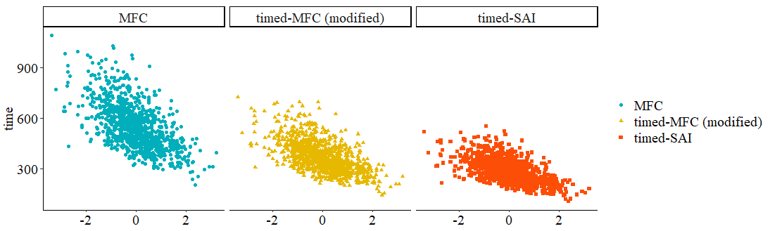
- scatter plot
- line plot
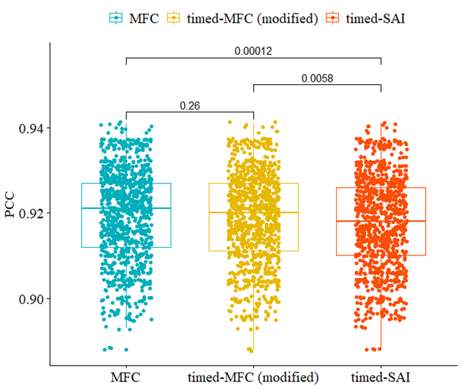
- boxplot with significant test
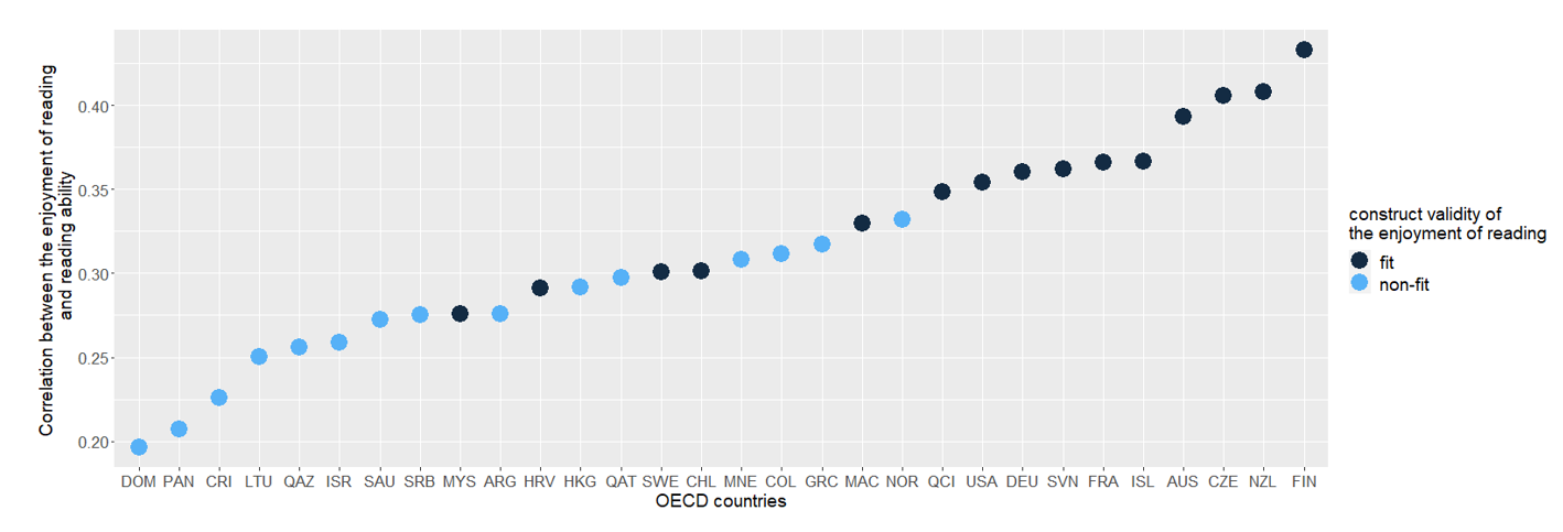
- order the points according to a particular variable
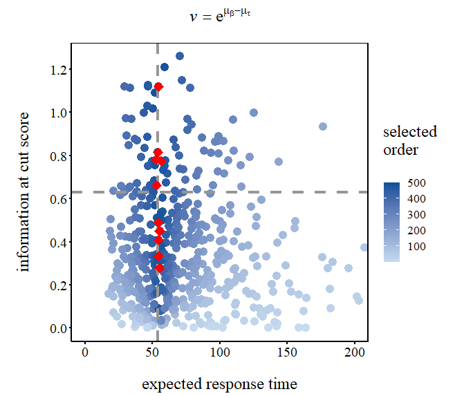
- highlight key data points
- insert texts and lines
- modify the shape or color
- scatter plot
- line plot
- boxplot with significant test
library(ggplot2)

# The first six rows of the data are showed below.
head(datause)
   method      theta     time
1    MFC   -1.2070657 826.5765
2    MFC    0.2774292 501.9339
3    MFC    1.0844412 607.5252
4    MFC   -2.3456977 621.7279
5    MFC    0.4291247 448.1083
6    MFC    0.5060559 725.4090

ggplot(datause, aes(x = theta, y = time))+
  geom_point(aes(color = method, shape = method))+
  scale_color_manual(values = c("#00AFBB", "#E7B800", "#FC4E07"))+

  # If you want to separate each group like I did, try the line below.
  facet_wrap(~method, ncol = 3, nrow = 1)+

  theme_set(theme_classic())+
  theme(legend.title = element_blank(),
        axis.text = element_text(size = 12, family="serif"),
        axis.title = element_text(size = 14, family="serif"),
        axis.title.x = element_blank(),
        axis.text.x = element_text(size = 15, family="serif", color = "black"),
        axis.text.y = element_text(size = 15, family="serif", color = "black"),
        plot.title = element_text(size = 14, family="serif"),
        legend.text = element_text(size = 15, family="serif"),
        strip.text = element_text(size = 15, family="serif"))

library(ggplot2)

# The first six rows of the data are showed below.
head(datause)
    nitems selection consistency   type  cut
1     20          RA   0.7541247  Rudner 25th
2     20       Theta   0.7671183  Rudner 25th
3     20         Cut   0.7671730  Rudner 25th
4     20          WM   0.7672108  Rudner 25th
5     20          GP   0.7671798  Rudner 25th
6     50          RA   0.8234817  Rudner 25th

plot.CC <- ggplot(data = datause,
                  aes(x = nitems, y = consistency, group = selection)) +
  geom_line(aes(colour = selection), size = 1) +
  geom_point(size = 2, aes(colour = selection, shape = selection)) +
  labs(x = "number of items", y = "Classification Consistency") +
  scale_x_continuous(breaks = c(20, 50, 70, 100)) +

  theme(text = element_text(size = 15, family = "sans"),
        axis.text.x = element_text(size = 15, face = "bold"),
        axis.text.y = element_text(size = 15, face = "bold"),
        plot.margin = unit(rep(3, 4), 'lines'),
        axis.title.x = element_text(vjust = -3),
        axis.title.y = element_text(vjust = 5),
        panel.spacing = unit(1, "lines"),
        legend.title = element_blank())

# We need to separate each plot according to the type of the index.
plot.CC + facet_grid(cut ~ type, scales = "free")
library(ggplot2)
library(ggpubr)      # This is the main character.

# The first six rows of the data are showed below.
head(datause)
    method   PCC
1     MFC    0.922
2     MFC    0.921
3     MFC    0.923
4     MFC    0.920
5     MFC    0.922
6     MFC    0.924

# Define the group pair that you want to test.
my_comparisons <- list(c("MFC", "timed-MFC (modified)"),
                       c("timed-MFC (modified)", "timed-SAI"),
                       c("MFC", "timed-SAI"))

# Great! We can make a boxplot first.
ggboxplot(datause, x = "method", y = "PCC",
	color = "method", palette = c("#00AFBB", "#E7B800", "#FC4E07"),

	# Add all your data onto the plot.
	add = "jitter"
	) +
	theme(legend.title = element_blank(),
	    axis.text = element_text(size = 12, family="serif"),
	    axis.title = element_text(size = 14, family="serif"),
	    axis.title.x = element_blank(),
	    axis.text.x = element_text(size = 15, family="serif", color = "black"),
	    axis.text.y = element_text(size = 15, family="serif", color = "black"),
	    plot.title = element_text(size = 14, family="serif"),
	    legend.text = element_text(size = 15, family="serif")
	    ) +
# Next, we can use t-test for comparision.
stat_compare_means(comparisons = my_comparisons, method = "t.test")- order the points according to a particular variable
library(ggplot2)
library(dplyr)

# The first six rows of the data are showed below.
head(datause)
   CNY code valid       corre modelFIT
1  QAZ   31     0   0.2560892  non-fit
2  ARG   32     0   0.2759617  non-fit
3  AUS   36     1   0.3932474      fit
4  CHL  152     1   0.3015014      fit
5  COL  170     0   0.3113862  non-fit
6  CRI  188     0   0.2261491  non-fit

# This step is to create a temporary data.frame to restore the order data.
# e.g, here, I want to re-order the data according to the correlation (i.e., corre)
tempDF <-
  infludata %>%
  arrange(corre)

head(tempDF)
   CNY code valid      corre modelFIT
1  DOM  214     0  0.1963621  non-fit
2  PAN  591     0  0.2072438  non-fit
3  CRI  188     0  0.2261491  non-fit
4  LTU  440     0  0.2500453  non-fit
5  QAZ   31     0  0.2560892  non-fit
6  ISR  376     0  0.2586625  non-fit

# Now you get the desired order, and you can start to plot.
order <- tempDF$CNY

ggplot(datause, aes(x = CNY, y = corre, color = modelFIT)) +
  geom_point(size = 6) +
  scale_x_discrete(limits = order) +
  scale_color_manual(values = c('#132b43','#56b1f7'))+
  labs(x = "OECD countries",
       y = "Correlation between the enjoyment of reading \n and reading ability") +
  labs(color = "construct validity of\nthe enjoyment of reading")+
  theme(legend.position = "right",
        legend.title = element_text(size = 14),
        legend.text = element_text(size = 14),
        axis.text = element_text(size = 13),
        axis.title = element_text(size = 14),
        plot.title = element_text(size = 14))
- highlight key data points
- insert texts and lines
- modify the shape or color
library(ggplot2)

# The first six rows of the data are showed below.
head(datause)
        info         ET        value
1  0.2070762  108.69578  0.003827824
2  0.2166885   92.40194  0.005731924
3  0.2430004   76.77980  0.010955015
4  0.7163323  102.87900  0.014836777
5  0.9668220  109.88926  0.017486031
6  0.1802682   19.84861  0.005187645

# I want to order the data points according to "value" and find the top 10 points,
# so I first create a new variable "ord" to signal the desired order.
datause$ord = findInterval(datause$value, sort(datause$value))

# Then, I can get my key points.
# (You can skip this if you have known your key points)
key <- datause[order(datause$ord, decreasing = T), ][1:10, ]

# Now my data was like:
head(datause)
        info         ET        value    ord
1  0.2070762  108.69578  0.003827824     89
2  0.2166885   92.40194  0.005731924    130
3  0.2430004   76.77980  0.010955015    216
4  0.7163323  102.87900  0.014836777    257
5  0.9668220  109.88926  0.017486031    283
6  0.1802682   19.84861  0.005187645    121

# I also define a horizontal line at y-axis.
y_med <- (max(datause$info)-min(datause$info))/2

# Finally, we can start to plot.
pe <- ggplot(datause, aes(ET, info)) +
        geom_point(aes(colour = ord), size = 4) +

        # As I did here, you can add additional lines to the plot.
        geom_hline(yintercept = y_med, color = "#969696", size = 1.5, linetype = "dashed")+
        geom_vline(xintercept = 54, color = "#969696", size = 1.5, linetype = "dashed")+

        # Here, we can highlight the key points.
        geom_point(data = as.data.frame(cbind(ET = key$ET, info = key$info)), aes(ET, info),
                   color = "red", shape = 18, size = 5) +

        # Listed below are some codes to make the plot look prettier.
        labs(x = "expected response time", y = "information at cut score",
             title = expression(italic(v) == e^paste(mu[beta]-mu[tau]))) +
        scale_y_continuous(breaks = seq(0, 1.2, 0.2))+
        scale_color_gradient(low = "#c6dbef", high = "#08519c") +
        labs(colour="selected\norder\n")+
        theme_minimal()+
        theme(panel.grid = element_blank(),
              panel.border = element_rect(fill = NA, color="black", size = 1, linetype = "solid"),
              axis.line.x = element_line(linetype = 1, color = "black", size = 1),
              axis.line.y = element_line(linetype = 1, color = "black", size = 1),
              axis.ticks.x = element_line(color = "black", size = 1),
              axis.ticks.y = element_line(color = "black", size = 1),
              axis.title.x = element_text(margin = margin(t = 20), size = 18, family = "serif"),
              axis.title.y = element_text(margin = margin(r = 20), size = 18, family = "serif"),
              plot.title = element_text(margin = margin(b = 20), hjust = 0.5, size = 18, family = "serif"),
              legend.position = "right",
              legend.title = element_text(size = 14, family = "serif"),
              axis.text = element_text(size = 15, color = "black", family = "serif"),
              legend.text = element_text(size = 13, family = "serif"))
pe + coord_fixed(ratio = 160, xlim = c(0, 200))
library(ggplot2)
library(ggridges)
library(hrbrthemes)
# The first six rows of the data are showed below.
head(datause)
th lnL
1 -3.00 -74.94047
2 -2.99 -74.64811
3 -2.98 -74.35579
4 -2.97 -74.06350
5 -2.96 -73.77125
6 -2.95 -73.47904
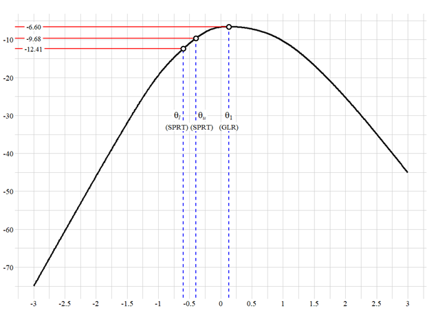
# This is our base plot, just a parabola.
p <- ggplot(datause, aes(x = th, y = lnL)) +
geom_line(color = "black", size = 1.5, alpha = 0.9, linetype = 1) +
scale_x_continuous(breaks = seq(-3, 3, 0.5), labels = seq(-3, 3, 0.5)) +
scale_y_continuous(breaks = seq(-80, 10, 10), labels = seq(-80, 10, 10)) +
theme_ipsum() +
theme(axis.text.x = element_text(size = 15, family="serif", color = "black"),
axis.text.y = element_text(size = 15, family="serif", color = "black")) +
xlab(" ") +
ylab(" ") +
ggtitle(" ") +
# Next, you can include some guidelines on the x-axis and y-axis using different colors.
# The setting of value is totally up to you.
geom_segment(x = -0.4, xend = -0.4, y = -100, yend = datause$lnL[261],
color = "blue", linetype = 2, size = 1)+
geom_segment(x = -0.6, xend = -0.6, y = -100, yend = datause$lnL[241],
color = "blue", linetype = 2, size = 1)+
geom_segment(x = datauseth[which.max(datauseth[which.max(datauselnL)], xend = datauseth[which.max(datauseth[which.max(datauselnL)],
y = -100, yend = max(datause$lnL),
color = "blue", linetype = 2, size = 1)+
geom_segment(x = -0.4, xend = -4, y = datauselnL[261],yend=datauselnL[261], yend = datauselnL[261],
color = "red", linetype = 1, size = 1)+
geom_segment(x = -0.6, xend = -4, y = datauselnL[241],yend=datauselnL[241], yend = datauselnL[241],
color = "red", linetype = 1, size = 1)+
geom_segment(x = datauseth[which.max(datauseth[which.max(datauselnL)], xend = -4,
y = max(datauselnL),yend=max(datauselnL), yend = max(datauselnL),
color = "red", linetype = 1, size = 1)
# You are encouraged to define the texts you want to add and their locations before the next step.
annotation1 <- data.frame(x = c(-3, -3, -3),
y = c(datauselnL[261],datauselnL[261], datauselnL[241], max(datause$lnL)),
label = c("-9.68", "-12.41", "-6.60"))
annotation2 <- data.frame(x = c(-0.7, -0.3, datauseth[which.max(datauseth[which.max(datauselnL)]),
y = c(-33, -33, -33),
label = c("(SPRT)", "(SPRT)", "(GLR)"))
# The merits of this is obvious.
# You can easily include those annotations through geom_label.
p + geom_label(data = annotation1, aes(x = x, y = y, label = label),
size = 5, family = "serif",
label.size = NA) +
geom_label(data = annotation2, aes(x = x, y = y, label = label),
size = 5, family = "serif",
label.size = NA) +
# But life isn't always smooth sailing,
# even so, if you also need to label some formulae, you can add them in this way.
annotate("label", x = -0.7, y = -30, label = expression(italic(theta[l])),
size = 6, family = "serif", label.size = NA)+
annotate("label", x = -0.3, y = -30, label = expression(italic(theta[u])),
size = 6, family = "serif", label.size = NA)+
annotate("label", x = datauseth[which.max(datauseth[which.max(datauselnL)], y = -30,
label = expression(italic(theta[1])),
size = 6, family = "serif", label.size = NA)+
# The codes below are used to make three points stand out.
# If you do not need to do so, feel free to skip this part.
annotate("point", x = -0.6, y = datause$lnL[241], size = 5)+
annotate("point", x = -0.4, y = datause$lnL[261], size = 5)+
annotate("point", x = datauseth[which.max(datauseth[which.max(datauselnL)], y = max(datause$lnL), size = 5)+
annotate("point", x = -0.6, y = datause$lnL[241], size = 3, color = "#ffffff")+
annotate("point", x = -0.4, y = datause$lnL[261], size = 3, color = "#ffffff")+
annotate("point", x = datauseth[which.max(datauseth[which.max(datauselnL)], y = max(datause$lnL), size = 3, color = "#ffffff")
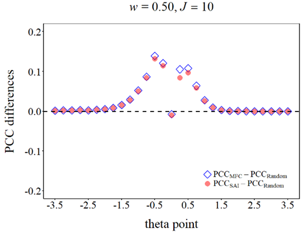
library(ggplot2)

# The first six rows of the data are showed below.
head(datause)
   theta    PCC method
1  -3.50 0.0017    MFC
2  -3.25 0.0021    MFC
3  -3.00 0.0022    MFC
4  -2.75 0.0029    MFC
5  -2.50 0.0022    MFC
6  -2.25 0.0038    MFC

# If your label name includes formulae, defining it as a variable will make things easier.
labelname <- c(expression(PCC[MFC] - PCC[Random]), expression(PCC[SAI] - PCC[Random]))

# Now we can start to plot.
w05 <- ggplot(datause)+
  geom_point(aes(x = theta, y = PCC, shape = method, col = method, alpha = method),
             size = 5, stroke = 1.5)+
  geom_hline(yintercept = 0, size = 1.3, linetype = "dashed")+

  # Here is the point, you can define different shapes and colors for different groups.
  scale_shape_manual(values = c(5, 16),
                     labels = labelname)+
  scale_color_manual(values = c("blue", "red"),
                     labels = labelname)+
  scale_alpha_manual(values = c(0.8, 0.5),
                     labels = labelname)+

  # Listed below are codes to limit the range of x-axis and y-axis.
  scale_y_continuous(limits = c(-0.2, 0.2), breaks = seq(-0.2, 0.2, 0.1))+
  scale_x_continuous(breaks = seq(-3.5, 3.5, 1))+

  # Listed below are some codes to make the plot look prettier.
  labs(x = "theta point", y = "PCC differences",
       title = bquote(paste(italic(w), " = 0.50, ", italic(J) == .(Ji))))+
  theme_minimal()+
  theme(panel.grid = element_blank(),
        panel.border = element_rect(fill = NA, color="black", size = 1, linetype = "solid"),
        axis.line.x = element_line(linetype = 1, color = "black", size = 1),
        axis.line.y = element_line(linetype = 1, color = "black", size = 1),
        axis.ticks.x = element_line(color = "black", size = 1),
        axis.ticks.y = element_line(color = "black", size = 1),
        axis.title.x = element_text(margin = margin(t = 20), size = 30, family = "serif"),
        axis.title.y = element_text(margin = margin(r = 20), size = 30, family = "serif"),
        plot.title = element_text(margin = margin(b = 20), hjust = 0.5, size = 30, family = "serif"),
        axis.text = element_text(size = 25, color = "black", family = "serif"),

        legend.position = c(.78, .12),
        legend.text = element_text(size = 20, family = "serif", hjust = 0),
        legend.title = element_blank())
w05 + coord_fixed(ratio = 12)
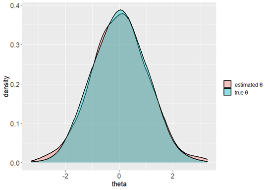
library(ggplot2)

# The first six rows of the data are showed below.
head(datause)
       type       theta
1 estimated  0.02181399
2 estimated  0.50863802
3 estimated  0.55536742
4 estimated -0.09117160
5 estimated -0.60815771
6 estimated -0.66477364

ggplot(data = datause, aes(x = theta, group = type, fill = type)) +

  # You can modify the color and transparency here.
  geom_density(adjust = 1.5, alpha = 0.4, size = 0.75) +

  theme(text = element_text(size = 15, family = "sans"),
        axis.text.x = element_text(size = 15),
        axis.text.y = element_text(size = 15),
        legend.title = element_blank())