
Tutorial: A Very Very Quick Guide for R
December 15, 2021
When we first come up with a plan to learn something new, it is more likely for us to keep working toward that goal if we get positive feedback immediately. Now! The prompt feedback you are looking for when learning R is here! After reading this article, you surely will be equipped with the ability to start your own project and the paintbrush to draw a bigger picture. Let's start!
Before we start our journey, we should make sure that we have brought enough "water and food". Downloading the following basic components in advance could prevent you from being stuck in various problems, such as not having RStudio open or certain packages not working.
- R (this is the heart): https://www.r-project.org/
- RStudio (this is a beautiful coat for R): https://www.rstudio.com/
- Rtools (it can provide resources for building packages): https://cran.r-project.org/bin/windows/Rtools/
The first question we need to address is: where can I code? A fast and direct answer is: RStudio. As you can see in the figure on the left side, the basic R is elegant and simple, but it may be too austere to write codes in an efficient way. Using RStudio can remedy this limitation with regard to code completion, viewing changes in real-time, etc.
When we open the RStudio, we can see four areas: editor window at the top left, working environment / history at the top right, console window at the bottom left, and files / plots / packages at the bottom right. To capture the function of each area, you can try to imagine that you are a director who is writing a script for a wonderful play. The editor window is where you write your script; The working environment is a greenroom for your actors; The console window is a stage where you can enjoy the performance; The plots are stage photos of your actors. (remember to spell the name of your actors correctly if you want them to perform for you :D)
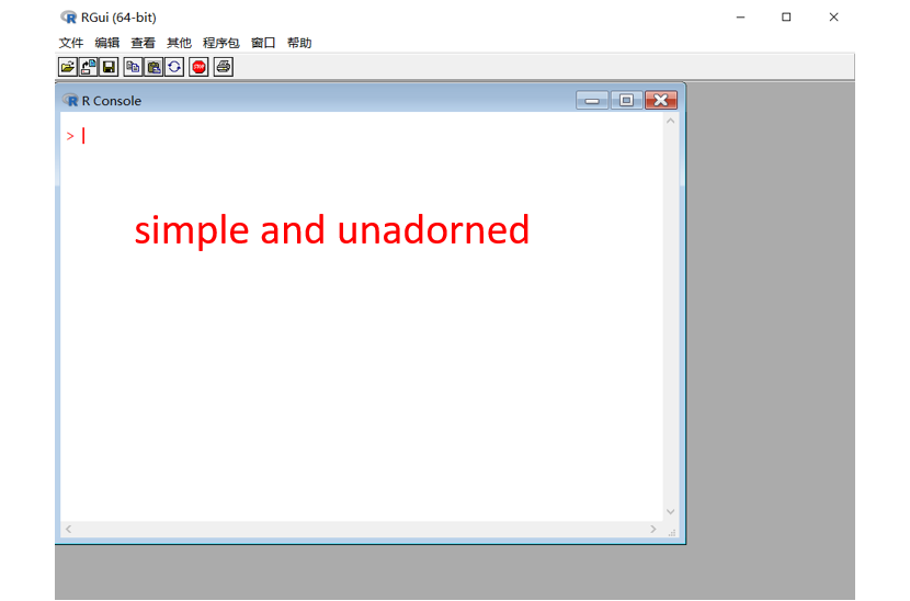
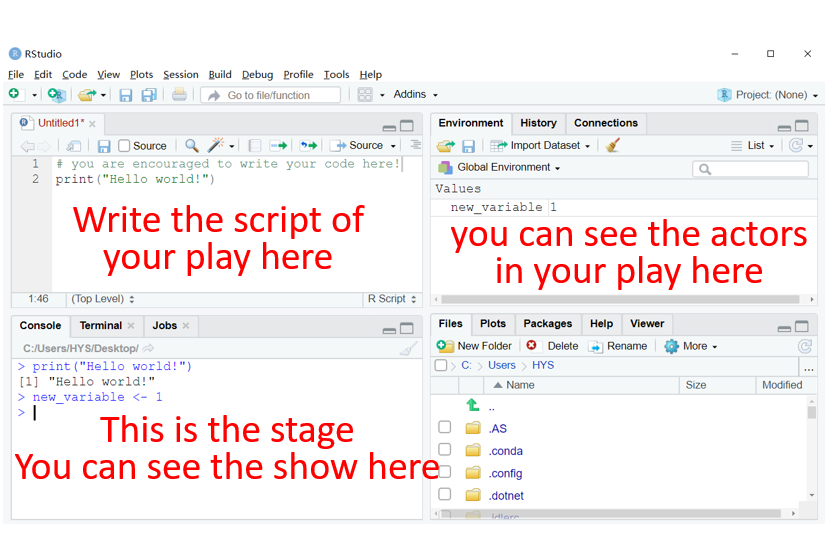
(1) Left: R Gui. (2) Right: RStudio.
Now let's get familiar with RStudio and find out how we can write our first script. It would be great if you open your RStudio and try to type in the lines below into your editor window.
# --------------------- get familiar with R ----------------------
##  run the code
# 1. If you want to run a single line of code,
#    you can move the cursor to that location and press: CTRL + ENTER
#    you can also click "Run" on the top right of this window
print("Press ctrl + enter to execute this line in the console")
print("Excellent! You made it!")

# 2. If you want to run the whole script, you can press: CTRL + ALT + R
# 3. If you want to rerun the some commands,
#    you can press the "up" arrows on your keyboard in the console window

## define variables
birth <- 1989          # This symbol <- assigns a value (1989) to a variable (birth)*
year  <- 2021          # You can press: "ALT" + "-" to obtain it in a quick way
age   <- year - birth  # You are allowed to create a new variable with the old ones

# Watch the environment window at the top right! Can you see your actors?

# You should bear in mind that the four variables listed below are four different objects.
# (it means that you should pay four salaries for these employees! just kidding)
object1  <- 1
Object1  <- 2
object.1 <- 3
object_1 <- 4

# These names are not allowed in R
1object  <- 1          # It can't start with a number
object 1 <- 1          # There must be No Space within a name

# You can fire all your actors with this line (clear the environment)
rm(list = ls())
*Some people may wonder why not use "birth = 1989"? You can do so because both of them do the same thing. The main difference between "=" and "<-" is that the former will produce a local variable (like a temporary employee) while the latter will bring you a global variable (like a permanent employee).
After knowing where we can code, we cannot wait to figure out what stuff we are going to handle. Basically, as shown in Table 1, we will encounter Logical, Numeric, Integer, Character, and Factor data (complex and raw data are relatively uncommon).
Table 1. How your data may look.
| Type | Example | Code |
| Logical | TRUE, FALSE | var <- FALSE |
| Numeric | 1, 299, 2.33, 0.134 | var <- 2.33 |
| Integer | 2L, 34L, 0L | var <- 666L |
| Character | "Hello" | var <- "Hello" |
| Factor | A B C Levels: A B C A B C Levels: A < B < C |
var <- factor(c("A", "B", "C")) var <- factor(c("A", "B", "C"), ordered = T) |
| Complex | 3 + 2i | var <- 3 + 2i |
| Raw | "Hello" is stored as: 48 65 6c 6c 6f | var <- charToRaw("Hello") |
If I only have only one element, like var = 2.33, I can manipulate this element with "var". But if I have thousands of data points, should I create var1, var2, ..., and var1000 to hold my data? Thanks to R Core Team, we do not have to do so. There are five data structures that can alleviate our burden.
(a) Vector. It is one-dimensional, and all data have the same mode (e.g., all are numeric). (b) Matrix. Each data point has two features and the same mode. (c) Array. More than two dimensions and still, all data have the same mode. (d) Data frame. Upgraded version for matrix, being amenable to different modes. (e) List. The ultimate boss or hodge-podge, embracing all kinds of data.
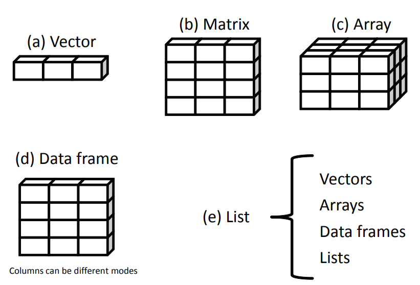
From R in Action, a terrific book detailing almost every aspect of R.
# -------------------- basic data structure ---------------------
## Here are examples for different modes of data
logic <- FALSE
logic <- T
num <- 2.33
int <- 666L
chr <- "Hello"
fac <- factor(c("A", "B", "C"), ordered = T)     # ordered factor
fac <- factor(c("male", "female"))               # unordered factor

## Vector: one-dimensional data with the same mode
num.vector <- c(1, 2, 3)
chr.vector <- c(1, 2, 3, "four")

# You can create a vector in various way.
vec.c <- c(1:9)
vec.seq     <- seq(from = 1, to = 9)
vec.seq.odd <- seq(from = 1, to = 9, by = 2)
vec.rep     <- rep(c(1:9), times = 2)
rep(c(1:9), each = 2)

# You can select a particular element in your vector with [ ]
vec.rep[3]

## Matrix: two-dimensional data with the same mode
## (noted that each colomn should contain the same length of elements)
mat.col <- matrix(data = c(1:9), nrow = 3, ncol = 3)              # the default setting is to fill the matrix by columns
mat.row <- matrix(data = c(1:9), nrow = 3, ncol = 3, byrow = T)   # you can change the setting to fill it by rows

# You can refer to the element in row x and colomn y with [x, y]
# Also, you can identify the xth row or yth colomn with [x, ] / [, y]
mat.row[2, 3]
mat.row[2, ]
mat.row[, 3]

## Array: for high dimensional data

# Here is an example for three-dimensional data
arr <- array(c(1:18), c(3, 3, 2))
arr

# The extraction for array is similar with Matrix
# (Let's try to figure out which number is corresponding to the height :D)
arr[2, 3, 2]

## Date.frame: it can hold different modes of data (one- or two-dimensional). Each colomn should contain the same length of elements.
## (it will be the most regular structure you will use)
participant <- data.frame(
                          ID  = c("sub_01", "sub_02", "sub_03", "sub_04"),
                          age = c(20, 21, 20, NA),
                          gender = factor(c("M", "F", "M", "F")),
                          treatment = c(F, F, T, T)
                          )
participant

# The extraction for data frame is also similar with Matrix
participant[1, 2]
participant[1, ]
participant$age

## List: it is so flexible that you can include everything here.
## (the length of element is also free)
listdata <- list(logic, num, chr, vec.c, mat.col, participant)
listdata
listdata[[5]][2, 3]
Now you surely have known how to "type in" your data by hand, you can also import your data into R directly from other sources. What is more, after analyzing your data, you may want to store your results timely. Rest assured, it is as simple as getting an elephant in a fridge. So, let's move on to see how to achieve this!
# ---------------------- read and write data -----------------------
## The fist step: know your working dictionary
getwd()
setwd("D:/Rwork")     # You should use a slash "/" instead of a backslash "\"
getwd()

## The second step: read your data

# 1. You can realize this goal using read.XXX
response <- read.csv(file = "response_matrix.csv")

# 2. You can also click the "import Dateset" at the top right
#    or "files" at the bottom right

## The third step: write your data
write.csv(x = participant, file = "participant.csv")

# This package can be used to read and write data from EXCEL
install.packages("openxlsx")
library(openxlsx)
exceldata <- read.xlsx(xlsxFile = "DataExample.xlsx")
write.xlsx(x = exceldata[, -1], file = "DataExample_minver.xlsx")

# This package can be used to read and write data from SPSS
install.packages("haven")
library(haven)
spssdata <- read_sav(file = "DataExample_SPSS.sav")
write_sav(data = na.omit(spssdata), path = "DataExample_SPSS_cleanver.sav")
(The example data can be downloaded here.)
Congratulations to you! You have the knowledge of RStudio and can employ your own data onto it (you are extremely close to success)! Since we have put our data in R, the final question awaited to be answered is: how can we analyze our data? Here we come to the core part of our codes. We will first cut our teeth in trying to do some basic operations on our data, and then we will go through two fundamental components (i.e., control flow and function) you will need when you do your own programming. Let's move ahead on our journey!
The first part is to get warm up by learning some basic operators in R. It would be a great notion to meet some actors we created before. Run the codes below and reveal the output by yourself.
# -------------------- basic operations ---------------------

## Arithmetic operators
1 + 1       # add
1 - 1       # subtract
2 * 2       # multiply
3 / 3       # divide
4 ^ 4       # power
4 ** 4      # power
5 %% 3      # remainder
5 %/% 3     # integer division

vec.rep
vec.rep + 1
vec.rep * 2

# When adding two vectors with different lengths, if the length of the longer one is an integral multiple of the shorter one,
# R will repeat the shorter vector for you.
vec.rep + c(1, 2, 3)
# But if the longer one's length is not a multiple of the other, there will be an error.
vec.rep + c(1, 2, 3, 4)

mat.row
mat.row * mat.row        # multiplying the corresponding elements in each matrix
mat.row %*% mat.row      # matrix multiplication
rowMeans(mat.row)        # compute row mean: (1+2+3)/3
colMeans(mat.row)        # compute column mean: (1+4+7)/3

## Logical operators
2 > 1
2 < 1
2 == 1         # strictly equal to
2 != 1         # not equal to
2 >= 2         # greater than or equal to

c(1,2,3) == 1
c(1,2,3) == c(1,2,3)

(2>1) & (3>1)  # and
(2>1) & (1>3)

(2>1) | (3>1)  # or
(2>1) | (1>3)

# For "&&" and "||", they will immediately move further once the statement is decisive enought.
if(FALSE && print(1)) {print(2)} else {print(3)}      # Command "print(1)" will be skipped
if(FALSE &  print(1)) {print(2)} else {print(3)}

if(TRUE || print(1)) {print(2)} else {print(3)}       # Command "print(1)" will be skipped
if(TRUE |  print(1)) {print(2)} else {print(3)}
Now comes the second part. So far, we have our actors right on the stage, and we can organize the play we wrote step-by-step by executing our script from the top to the bottom. The appearance of our actors, however, may be more flexible instead of being presented in a plain and flat way. Some actors may appear only when certain music is cued while some actors may need to show up over and over again during the first movement.
In other words, rather than allowing your codes to flow naturally, in some cases, you may want to designate a direction if some conditions are met, or require a circulating flow. Consequently, the question then becomes: how can we control the flow of our codes? Two powerful constructs, conditional execution and looping, are readily harnessed to satisfy our ambition.
# ---------------------- conditional execution -----------------------
## if statements

# if a given condition is true, this control structure will execute a statement you assigned
input <- 3
if(input%%2 == 0){                 # This is the condition needed to be tested
  print("It is an even.")          # R will execute this line if the condition is met
}

if(input%%2 == 0){
  print("It is an even.")
}else{                             # R will execute this part if the condition is not met
  print("It is an odd.")           # You can omit this part if you do not need it as in the former example
}

input <- 3.4
if(input%%2 == 0){
  print("It is an even.")
}else if(input%%2 == 1){           # More detailed conditions can be included in this way
  print("It is an odd.")
}else{
  print("It is not an integer.")
}

# You can apply "ifelse" when you want to enter more than one element
input <- c(3, 4)
ifelse(test = (input%%2 == 0),
       yes = "It is an even.",
       no = "It is an odd.")

## The do's and don'ts
# 1. If you have multiple conditions, please always ensure them to be mutually exclusive.
# 2. Please always try to enter different inputs to check whether you can get the desired output.


# ---------------------- repetition and looping -----------------------
## for: You know where is the end

# When you want to execute a statement repetitively, it would be tedious to enter the same codes over and over again.
# If you have a sequence defining how many times R should execute your statement, the for-loop structure is advisable.
for (i in 1:5){                # R will run through i = 1, i = 2, ..., i = 5
  print(i)                     # then, the i value will be printed out in each run; that is, this line will be processed 5 times
}

for (i in c("A", "B", "C")){   # the sequence you want to go through can also be a vector of characters
  print(i)
}

## while: You have no idea about where is the end, but you do know what would be the time to stop

# If you do not know the exact sequence, but you incline to terminate the loop at a specific point, the while-loop structure is recommended.
# While loop can help you to execute the same statements until the condition is not met.
i <- 1                         # this is a counter
while(i < 6){                  # when the condition in the parenthesis is TRUE, R will keep executing the next statements in the brackets
  print(i)                     # that is, R will keep printing out i if i is less than 6
  i <- i + 1                   # also, the value of i will be increased by one after each run
}                              # this cycle will reach its end when i is lager than or equal to 6

## The do's and don'ts
# 1. You must make sure that there is an end point for while-loop, if not, it will keep going until reaching the end of the earth.
# 2. Looping constructs are the most time-consuming part of your program, you can try to replace them with "apply" function.
#    (It would be a long story so I am not going to cover this function here. Instead, you can Google "apply in R" to see more details).
Another fundamental component you will need in the journey is function. R has a gamut of packages containing diverse functions to help you realize your analysis of data. More importantly, you can even build your own function to carry out what you want personally! Let's see how to do so.
# ---------------------- function -----------------------
## How to use packages?

# The first step is to install packages if you haven't included them in R before.
install.packages("swirl")        # This is a marvelous package to learn R in R. I went through all sections in swirl when I learned R by myself.
install.packages("ggplot2")      # This is a powerful package to visualize your data.

# The second step is to load the package, and then the functions attached will be accessible.
library(ggplot2)

# When you encounters a problem, you can ask for help in these way:
# 1. It is really helpful to view the R document including the description, usage, examples, or other details of the package.
?ggplot2                         # Typing in a question mark before the package you want to get more information.
help("ggplot2")                  # You can also use the "help" function.
help("apply")

# 2. Another option is to search the help system if you cannot remember the exact name or want to receive the related information.
??ggplo                          # Typing in two question marks to call the help system.
help.search("ggplo")             # Or using the "help.search" function.


## How to introduce your own function?

# The main features:
# Say you would like to write a function praising someone.
praise <- function(yourname){                                         # The objects used in the function should be included here. Note that these objects are local to the function, so you will not see them in the global environment.
  # A function that prasies a specific person (You should annotate the purpose and usage of your function)
  print(paste(yourname, "is the best person I have ever met!"))       # This statement will give you a compliment.
}
praise(yourname = "Taylor")                                           # Now try this example in your R, replacing the input with your name!

# Next we move on to a more complex example.
# If your object always has the same value, you can include it as a default value.
praise <- function(yourname, agree = T){                              # Say we always agree that the name you input is a great person.
  print(paste(yourname, "is the best person I have ever met!"))
  if (agree == T){                                                    # In this case, we should evaluate whether the value you enter is met with your default value.
    print("I think so!")                                              # If the condition is TRUE, we should expect that this statement to be printed.
  }else{
    print("Beyoncé is the best!")                                     # Otherwise, this line will be printed.
  }
}
praise(yourname = "Taylor")                                           # Now let's run this function with the default value.
praise(yourname = "Taylor", agree = F)                                # Changing the default value to figure out what would happen.

# Here is a more realistic example, and you can write your function to calculate the variables you want!
likf <- function(th, re, a, b, D = 1.702) {     # Covering all objects here, and their name should be meaningful (it is usually an abbreviation of the full name). Here th = theta, re = response.
  # This is a function calculating an examinee's likelihood.
  pi <- 1 /(1 + exp(-D * a * (th - b)))         # This is a formula to calculate the probability of a correct answer.
  li <- prod(pi^re * (1 - pi)^(1 - re))         # "prod" returns the product of all the values in its arguments.
  return(li)                                    # Noticed that R will not print out the results if you do not ask for them, so you should like to use the "return" function or simply type in "li" at the end.
}

# Now try to run this example.
th <- 1
re <- c(1, 1, 0, 1)
a <- c(0.8, 0.9, 0.5, 0.9)
b <- c(0.5, 0.4, 1, 0.6)
likf(th, re, a, b)

## The do's and don'ts
# 1. You should include all objects used in the function within the parenthesis.
     Never trying to use objects from the global environment, though it works sometimes.
     This behavior will give you unexpected errors when you unintentionally miss something.
# 2. If you want to output more than one result or a value produced in the middle of the statements, you need to use the "return" function to tell R what you want;
     otherwise, R will only give you the last value produced in the statement.
# 3. If you do not point out the variables you input should be what object in the function, please arrange your variables in the same order as the function defined.
likf(re, th, a, b)                              # This will give you a wrong number as R confuses the object th with "re" and the object re with "th"!
likf(re = re, th = th, a = a, b = b)            # The confusion will be eliminated if you clarify the name of each object, so I recommend you always do so.
# 4. It is always instructive and advisable to view the function in the package you intend to use.
     You can gain a clear picture of the underlying codes of that function, and you can learn from the codes too!
install.packages("cacIRT")                      # This is a package used to calculate classification accuracy and consistency.
library(cacIRT)                                 # Thanks very much for Dr. Quinn N. Lathrop (2014)'s excellent job!
Rud.P                                           # You can scrutinize the codes of a function by taking out the parenthesis, that is, from "Rud.P()" to "Rud.P".
You have reached a milestone! All your data are well introduced to R, and you have a full-fledged programming structure. Your actors are ready for the show and the stage has been set up well. Before the show, we can involve some excellent sound and lighting effects: visualization. A clear and eye-catching plot is rewarding and can help clarify your results.
Let's take a look at two examples, and the resulting graphs are provided at the end of this section.
# ----------------------- visualization ------------------------
## Using "plot" to draw a scatter plot for estimates and true values!
theta  <- rnorm(1000)
est.th <- theta + rnorm(1000, 0, 0.5)
plot(theta, est.th)

# You can make it prettier by adjusting a broad selection of parameters
plot(theta, est.th,
     col = rgb(0.4, 0.4, 0.8, 0.6),             # change the color of your points
     pch = 16,                                  # choose specific symbol (or shape)
     cex = 1.3,                                 # size of the scatter point
     cex.lab = 1.5,                             # size of the axis label text
     cex.axis = 1.5,                            # size of the numbers on the tick marks
     family = "sans",                           # font style
     xlab = "true θ", ylab = "estimated θ",     # the label of x-axis and y-axis
     xlim = c(-3.5, 3.5), ylim = c(-3.5, 3.5))  # control the range of x-axis and y-axis
reg <- lm(est.th ~ theta)
abline(reg,
       lty = 1,           # type of line
       lwd = 2,           # width of line
       col = "red")       # color of line

## Now let us try to draw with ggplot2!
library(ggplot2)

# Initially, we should put our data in data.frame
ggplotdata <- data.frame(true = theta,
                         estimated = est.th)

# Then, we can call ggplot
ggplot(ggplotdata, aes(x = true, y = estimated)) +        # tell ggplot what data you would like to plot
       geom_point(col = rgb(0.4, 0.4, 0.8, 0.6)) +        # draw a scatter plot and define a color for the points
       geom_smooth(method = lm, color = "red", se = F)    # draw a regression line for your data points
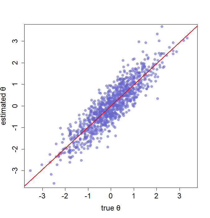
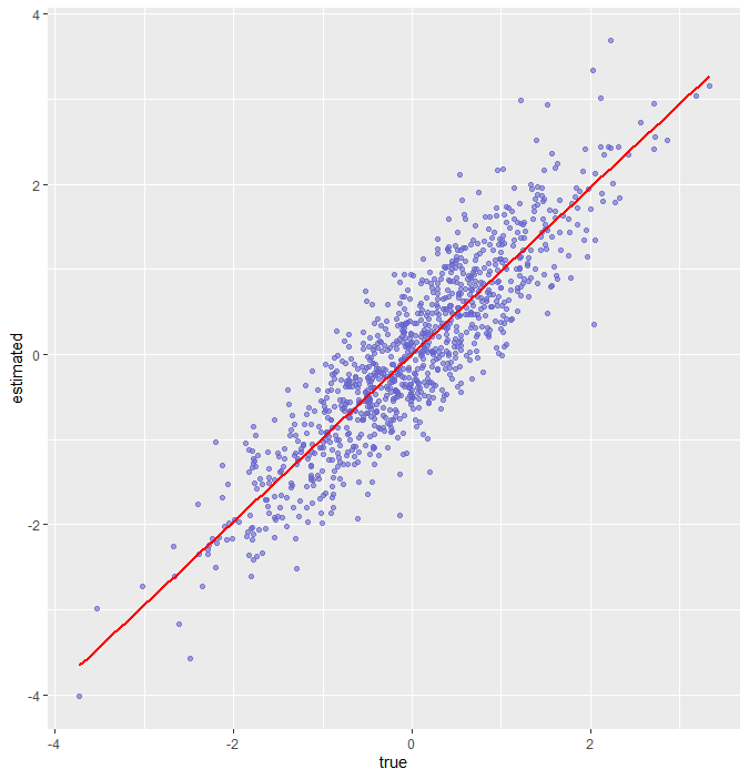
(1) Left: example 1 using standard plotting. (2) Right: example 2 using ggplot2.
(And now you may realize that it is important for us to adjust some parameters to adorn our graphs.)
Finally! You are a qualified R programmer from this moment! In previous sections, you have been familiar with the layout of RStudio and have found out how to execute your codes in R. Then, you are capable of importing and storing the data. More importantly, you can proceed well with the conditional and looping structures and are not limited to the existing functions! Since you have captured the whole framework, it is time for you to add more details to your own picture.
In addition, I have prepared some practical recommendations and resources to help you enjoy your R journey.
- Always annotating your codes is a priceless merit. Also, you can turn codes into comments through Ctrl + shift + C.
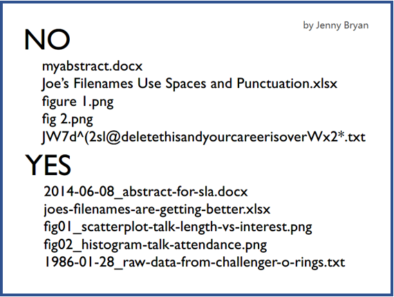
- The primary goal for all language is to communicate and share meaning, and computer language is no exception. So, naming your variables or files with substantial meaning is important.
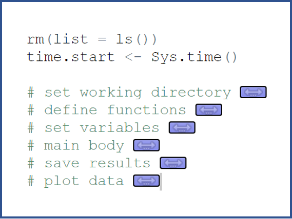
- A block structure helps shape a brisk coding experience.
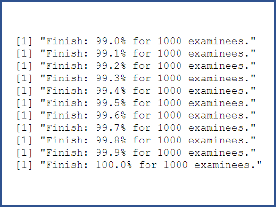
- A processing bar can mollify your agitated mind during the long run time of the program.
- The powerful R document: https://www.rdocumentation.org/
- This page will answer 99% of your questions: https://stackoverflow.com/
- Here are great codes to help you visualize your data: https://www.r-graph-gallery.com/
- Following stylistic guidelines can make your code readable: http://adv-r.had.co.nz/Style.html
- Google is your faithful friend!