The project framework

1. Define function
2. Set variables
   I set some variables used in this study and generated item and person parameters in this part.
3. Main body
   The estimation main body and the computation of seven evaluation criteria (i.e., bias and RMSE of ability, bias and RMSE of speed, M and SD of testing times, mean of testing overlap rate).
4. Save results
   Save results and return evaluation indexs and timecost to the console.

CAT with response time

Before we get started, it would be a good idea to clean our environment, record the starting time point, and set our working directory.

rm(list = ls())
time.start <- Sys.time()

# library packages ----------------------------------------
## This package can help you to produce samples from multivariate normal distribution
library(MASS)

# set working directory -----------------------------------
setwd("C:/Users/HYS/Desktop")         ## You need to modify to your WD

I introduced nine functions to implement the item selection methods, estimate examinees' abilities and speednesses, etc.
A. function1: itemInfo, compute Fisher information for dichotomous IRT model
B. function2: respon, generate response data for an examinee
C. function3: responTime, generate response time for an examinee
D. function4: selectRandom, Random selection method
E. function5: selectMFI, maximum Fisher information selection method
F. function6: selectGMIT, Generalized MIT method
G. function7: estMLE, estimate theta for an examinee with maximum likelihood method
H. function8: estEAP, estimate theta for an examinee with expected a posteriori method (as an interim substitute of MLE)
I. function9: estTau, estimate speed parameter for an examinee with maximum likelihood method

# define functions ----------------------------------------
itemInfo <- function(theta, a, b, c = 0, d = 1, D = 1.7){
  # only for dichotomous IRT model
  th <- theta
  it <- cbind(a, b, c, d)
  a <- it[, 1]
  b <- it[, 2]
  c <- it[, 3]
  d <- it[, 4]
  D <- D
  e <- exp(D * a * (th - b))
  Pi <- c + (d - c) * e/(1 + e)
  Pi[Pi == 0] <- 1e-10
  Pi[Pi == 1] <- 1 - 1e-10
  dPi <- D * a * e * (d - c)/(1 + e)^2
  
  P  <- Pi
  dP <- dPi
  Q  <- 1 - P
  Ii <- dP^2/(P * Q)
}

respon <- function(theta, a, b, c = 0, D = 1.7){
  ## To generate response data for an examinee
  ni <- length(a)
  if (length(c) == 1) {
    c <- rep(c, ni)
  }
  probs <- sapply(1:ni, function(i) {
    c[i] + (1 - c[i])/(1 + exp(-D * a[i] * (theta - b[i])))
  })
  respondata <- ifelse(test = probs >= runif(n = ni, min = 0, max = 1), yes = 1, no = 0)
}

responTime <- function(tau, alpha, beta){
  ## To generate response time for an examinee
  ni <- length(alpha)
  time <- sapply(1:ni, function(i) {
    rlnorm(n = 1, meanlog = beta[i] - tau, sdlog = 1/alpha[i])
  })
}

selectRandom <- function(itemFlag){
  ## To select items randomly
  nitemBank <- length(itemFlag)
  rand <- sample(seq(1, sum(itemFlag)), 1)
  id   <- (1:nitemBank)[itemFlag > 0][rand]
}

selectMFI <- function(itemFlag, theta, a, b, c = 0, d = 1, D = 1.7){
  ## To select items according to the order of Fisher information at current estimated theta
  info  <- itemInfo(theta = theta, a = a, b = b, c = c, d = d, D = D)
  ranks <- rank(info)
  keepRank <- sort(ranks[itemFlag > 0], decreasing = TRUE)[1]
  id <- which(ranks == keepRank & itemFlag == 1)
  
  ## items are selected randomly from those best ones
  if (length(id) > 1){
    id <- sample(id, 1)
  }else{
    id <- id
  }
}

selectGMIT <- function(itemFlag, v, w, theta, tau, alpha, beta, a, b, c = 0, d = 1, D = 1.7){
  ## To select items with GMIT method
  info <- itemInfo(theta = theta, a = a, b = b, c = c, d = d, D = D)
  ET   <- exp(beta - tau + 1/(2 * alpha^2))
  deno <- abs(ET - v)^w
  IT   <- info/deno
  ranks    <- rank(IT)
  keepRank <- sort(ranks[itemFlag > 0], decreasing = TRUE)[1]
  id <- which(ranks == keepRank & itemFlag == 1)
  
  ## items are selected randomly from the those best ones
  if (length(id) > 1){
    id <- sample(id, 1)
  }else{
    id <- id
  }
}

estMLE <- function (re, a, b, c = 0, D = 1.7, min = -4, max = 4){
  ## maximum likelihood estimates of theta for an examinee
  ## compute log-likelihood function
  logf <- function(x, r, a, b, c, D) {
    pi = c + (1 - c)/(1 + exp(-D * a * (x - b)))
    ll = r * log(pi) + (1 - r) * log(1 - pi)
    lf = sum(ll)
    return(lf)
  }
  ## find the optimal theta with max log-likelihood function
  th <- optimize(logf, lower = min, upper = max, maximum = TRUE,
                 r = re, a = a, b = b, c = c, D = D)$maximum
  return(th)
}

estEAP <- function(re, a, b, c = 0, D = 1.7, priorPar = c(0, 1), lower = -4, upper = 4, nqp = 40){
  ## expected a posteriori estimate of theta for an examinee
  it <- cbind(a, b, c)
  X  <- seq(from = lower, to = upper, length = nqp)
  
  ## compute likelihood function
  LL <- function(x, r, it, D) {
    a <- it[, 1]
    b <- it[, 2]
    c <- it[, 3]
    pi <- c + (1 - c)/(1 + exp(-D * a * (x - b)))
    lls <- pi^r * (1 - pi)^(1 - r)
    ll <- 1
    for (i in 1:length(a)) ll <- ll * lls[i]
    return(ll)
  }
  
  ## use normal distribution as the prior distribution
  num <- deno <- NULL
  for (i in 1:length(X)) num[i] <- X[i] * dnorm(X[i], priorPar[1], priorPar[2]) * LL(X[i], re, it, D)
  for (i in 1:length(X)) deno[i] <- dnorm(X[i], priorPar[1], priorPar[2]) * LL(X[i], re, it, D)
  
  th <- sum(num)/sum(deno)
  return(th)
}

estTau <- function(alpha, beta, logt){
  ## maximum likelihood estimates of speed for an examinee
  num  <- alpha^2 * (beta - logt)
  deno <- alpha^2
  speed <- sum(num)/sum(deno)
  return(speed)
}

Then, with the functions defined above, we can begin work on constructing a complete routine for CAT. To achieve this goal, we should first generate our examinees and the item bank, which are included in the "set variables" section. Later, a CAT with response time was presented in the "main body" section.

# set variables -------------------------------------------
nperson <- 1000
nitemBank <- 500
total.test.length <- 50
select.method <- c("Random", "MFI", "GMIT")
v <- 1
w <- 0.5
D <- 1.7

set.seed(13)
## generate item parameters
mu1 <- c(0.3, 0, 0)
sigma1 <- matrix(c(0.1, 0.15, 0,
                  0.15, 1, 0.25,
                  0, 0.25, 0.25), 3, 3)
itempara <- mvrnorm(n = nitemBank, mu1, sigma1)
a <- exp(itempara[, 1])
b <- itempara[, 2]
c <- rbeta(n = nitemBank, 2, 10)
alpha <- runif(n = nitemBank, min = 2, max = 4)
beta  <- itempara[, 3]

## generate person parameters
mu2 <- c(0, 0)
sigma2 <- matrix(c(1, 0.25, 0.25, 0.25), 2, 2)
personpara <- mvrnorm(n = nperson, mu2, sigma2)
theta <- personpara[, 1]
tau   <- personpara[, 2]

# main body -----------------------------------------------
estth.end <- esttau.end <- matrix(data = NA, nrow = nperson, ncol = length(select.method))
test.time <- matrix(data = NA, nrow = nperson, ncol = length(select.method))
ID.bank   <- matrix(data = NA, nrow = nperson, ncol = total.test.length * length(select.method))
eval.index <- matrix(data = NA, nrow = 7, ncol = length(select.method))

for (m in 1:length(select.method)){
  for (i in 1:nperson){
    test.length <- 0
    est.th <- est.tau <- 0
    item.Flag <- rep(1, nitemBank)
    response  <- response.time <- test <- NULL
    
    while(test.length < total.test.length) {
      ## randomly choose the first item
      if (test.length == 0) {
        item.ID <- selectRandom(itemFlag = item.Flag)
      }else{
        item.ID <- switch(m, selectRandom(item.Flag),
                          selectMFI(item.Flag, est.th, a, b, c),
                          selectGMIT(item.Flag, v, w, est.th, est.tau, alpha, beta, a, b, c))
      }
      item.Flag[item.ID] <- 0
      test.length <- test.length + 1
      
      ## generate reponse socre and response time
      response[test.length] <- respon(theta = theta[i], a = a[item.ID],
                                      b = b[item.ID], c = c[item.ID])
      response.time[test.length] <- responTime(tau = tau[i], alpha = alpha[item.ID],
                                               beta = beta[item.ID])
      test[test.length] <- item.ID
      
      ## estimate theta with MLE method (EAP as an interim substitute)
      if(test.length >= 5 && sum(response) != 0 && sum(response) != test.length){
        est.th <- estMLE(re = response, a = a[test], b = b[test], c = c[test], D = D)
      }else{
        est.th <- estEAP(re = response, a = a[test], b = b[test], c = c[test], D = D)
      }
      
      ## estimate speed parameter with MLE method
      est.tau <- estTau(alpha = alpha[test], beta = beta[test], logt = log(response.time))
    }
    estth.end[i, m]  <- est.th
    esttau.end[i, m] <- est.tau
    test.time[i, m]  <- sum(response.time)
    
    ## collect ID of selected items
    ID.bank[i, (1 + total.test.length * (m - 1)) : (total.test.length * m)] <- test
    
    ## progress bar
    print(paste("Finish: ", sprintf(fmt = '%0.1f', i/nperson * 100), "% for ", nperson,
                " examinees with ", select.method[m], " item selection method.", sep = ""))
  }
  
  ## compute evaluation indexs
  eval.index[1, m] <- mean(theta - estth.end[, m])            # bias of theta
  eval.index[2, m] <- sd(theta - estth.end[, m])              # RMSE of theta
  eval.index[3, m] <- mean(tau - esttau.end[, m])             # bias of speed parameter
  eval.index[4, m] <- sd(tau - esttau.end[, m])               # RMSE of speed parameter
  eval.index[5, m] <- mean(test.time[, m])                    # mean of testing times
  eval.index[6, m] <- sd(test.time[, m])                      # standard deviation of testing times
  
  # compute the mean of testing overlap rate
  item.overlap <- sapply(1:nitemBank, function(j){
    used.times <- sum(ID.bank[, (1 + total.test.length * (m - 1)) : (total.test.length * m)] == j)
    er <- used.times/nperson
  })
  eval.index[7, m] <- (nperson * sum(item.overlap^2)) / (total.test.length * (nperson - 1)) - 1/(nperson - 1)
}
							

The final part is to write your results. Let's see whether can you reach the same conclusion as Dr. Choe did. :D

# save results --------------------------------------------
## for theta
theta.result <- cbind.data.frame(estth.end, theta)
colnames(theta.result) <- c("Random", "MFI", "GMIT", "true_theta")
write.csv(x = theta.result, file = "est_theta.csv", row.names = FALSE)

## for speed parameter
tau.result <- cbind.data.frame(esttau.end, tau)
colnames(tau.result) <- c("Random", "MFI", "GMIT", "true_tau")
write.csv(x = tau.result, file = "est_tau.csv", row.names = FALSE)

## for test time
test.time.result <- test.time
colnames(test.time.result) <- c("Random", "MFI", "GMIT")
write.csv(x = test.time.result, file = "test_time.csv", row.names = FALSE)

## for evaluation indexs
eval.index.results <- eval.index
colnames(eval.index.results) <- c("Random", "MFI", "GMIT")
rownames(eval.index.results) <- c("bias_th", "RMSE_th", "bias_tau", "RMSE_tau",
                                  "test_time_mean", "test_time_sd", "test_overlap_mean")
write.csv(x = eval.index.results, file = "evaluation_indexs.csv", row.names = TRUE)

timeCost <- Sys.time() - time.start

## return the results to the console
print(list(studyResults = eval.index.results, timeCost = timeCost))
							

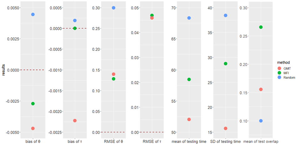
The scatter plot of the results.

Now you can use these codes to try using response times and build your own CAT!
Also, feel free to ask me any questions.