The project framework

1. function1: Newtons, Newton-Raphson method of theta estimation for 2PLM (with the implement of downhill algorithm)
2. function2: GridSearch, Grid-Search method of theta estimation for 2PLM (an option for the estimation of score of 0 or full scores)

1. plot estimate theta results
2. save results
3. return bias, RMSE and timecost to the console

MLE with the downhill algorithm

Before we get started, it would be a good idea to clean our environment, record the starting time point, and set our working directory.

rm(list = ls())
time.start <- Sys.time()

# library packages ----------------------------------------
## This package can help you to produce gorgeous graphs
library(ggplot2)

# set working directory -----------------------------------
setwd("C:/Users/HYS/Desktop")         ## You need to modify to your WD

Next, let's take a close look at the core functions.

# define functions ----------------------------------------
Newtons <- function(theta0, response, a, b, D = 1.702, lamda = 1, ep = 1e-08, maxiter = 500){
  ## Newton-Raphson method of theta estimation for 2PLM
  th <- theta0
  re <- response
  niter <- 0
  delta <- ep + 1

  while (delta >= ep && niter <= maxiter) {
    niter <- niter + 1
    
    ## 2PL model
    Pi <- 1 /(1 + exp(-D * a * (th - b)))
    Pi[Pi == 0] <- 1e-10
    Pi[Pi == 1] <- 1 - 1e-10
    Q <- 1 - Pi
    fx <- sum(D * a * (re - Pi))       # first derivative, i.e., g(θ)
    dfx <- -D^2 * sum(a^2 * Pi * Q)    # second derivative, i.e., g'(θ)
    
    ## detect if the slope is zero
    if (dfx == 0) {
      warning("Slope is zero!")
      break
    }

    delta <- lamda * fx/dfx
    
    ## implement the downhill algorithm
    j <- 0
    Pi1 <- 1 /(1 + exp(-D * a * (th - delta - b)))
    fx1 <- sum(D * a * (re - Pi1))     # compute g(θk+1)
    fx0 <- fx                          # compute g(θk)
    while (abs(fx1) >= abs(fx0)) {
      j <- j + 1
      lamda <- lamda/(2^j)
      delta <- lamda * fx/dfx
      Pi1 <- 1 /(1 + exp(-D * a * (th - delta - b)))
      fx1 <- sum(D * a * (re - Pi1))
    }
    
    th <- th - delta
  }
  
  ## detect the misconvergence
  if (niter > maxiter) {
    warning("Maximum number of iterations was reached.")
  }
  return(list(root = th, niter = niter, estim.prec = delta))
}

GridSearch <- function(response, a, b, D = 1.702, upper = 4, lower = -4, stepsize = 1e-03){
  ## Grid-Search method of theta estimation for 2PLM
  th <- seq(from = lower, to = upper, by = stepsize)
  np = length(th)
  
  ## compute log-likelihood function
  logf <- function(x, r, a, b, D) {
    pi = 1/(1 + exp(-D * a * (x - b)))
    ll = r * log(pi) + (1 - r) * log(1 - pi)
    lf = sum(ll)
    return(lf)
  }
  
  ## for each theta in [lower, upper]
  lnL <- sapply(1:np, function(i){
    logf(x = th[i], r = response, a = a, b = b, D = D)
  })
  th <- th[order(lnL, decreasing = TRUE)]
  estth <- th[1]
}
							

Are you ready for estimating our example data? Here we go!

# main body -----------------------------------------------
## read data
response <- read.table("response_matrix.txt")
theta    <- read.table("theta_parameter.txt")
itemPara <- read.table("item_parameter.txt")

## set variables
D <- 1.702
lamda <- 1
upper <- 4
lower <- -4
epsilon <- 1e-08
maxiter <- 1000
stepsize <- 1e-05

## estimate theta for all examinees
a <- itemPara[, 1]
b <- itemPara[, 2]
nperson <- dim(response)[1]
nitem   <- dim(itemPara)[1]

est.th <- array(data = NA, dim = nperson)
for (i in 1:nperson) {
  score <- sum(response[i, ])
  
  ## check score of 0 or full scores
  if(score == 0) {
    est.th[i] <- -3
    ## if we want to use the Grid-Search method, that is:
    ## est.th[i] <- GridSearch(response = response[i, ], a = a, b = b, D = D,
    ##                         upper = upper, lower = lower, stepsize = stepsize)
  }else if (score == nitem){
    est.th[i] <- 3
  }else{
    theta0 = log((score) / (nitem - score))
    est.th[i] <- Newtons(theta0 = theta0, response = response[i, ], a = a, b = b, D = D,
                         lamda = lamda, ep = epsilon, maxiter = maxiter)$root
  }
  
  ## boundary manipulation
  if(est.th[i] > upper) {
    est.th[i] <- upper
    print(paste("The ", i, "th estimated theta is out of range.", sep = ""))
  }else if (est.th[i] < lower) {
    est.th[i] <- lower
    print(paste("The ", i, "th estimated theta is out of range.", sep = ""))
  }
  
  ## progress bar
  print(paste("Finish: ", sprintf(fmt = '%0.1f', i/nperson * 100), "% for ",
              nperson, " examinees.", sep = ""))
}

## compute the indexs
bias <- mean(est.th - theta[, 1])
RMSE <- sd(est.th - theta[, 1])
							

After the estimation, we surely want to know the accuracy of our estimators. So, let's plot the estimated abilities and true values. Also, do not forget to save our results.

# plot estimate theta results -----------------------------
## generate a density plot
data <- data.frame(
  type = rep(x = c("estimated θ", "true θ"), each = nperson),
  theta = c(est.th, theta[, 1]))

pic <- ggplot(data = data, aes(x = theta, group = type, fill = type)) +
  geom_density(adjust = 1.5, alpha = 0.4, size = 0.75) +
  theme(text = element_text(size = 15, family = "sans"),
        axis.text.x = element_text(size = 15),
        axis.text.y = element_text(size = 15),
        legend.title = element_blank())
pic

# save results --------------------------------------------
result <- cbind.data.frame(est.th, theta)
colnames(result) <- c("est_theta", "true_theta")
write.csv(x = result, file = "est_theta.csv", row.names = FALSE)
timeCost <- Sys.time() - time.start

# return the results to the console -----------------------
print(list(bias = bias, RMSE = RMSE, timeCost = timeCost))
							

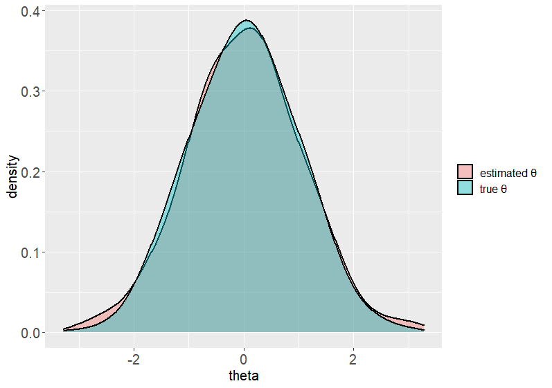
The density plot of the results.

You have done a terrific job! Now you can use these codes to estimate your own theta with your a and b parameters! Also, feel free to ask me any questions.